Weihrauch Reducibility as a Lens

A short while ago, we had CCA 2024 at Swansea, which I attended mostly because it was local and my supervisor was giving a talk. The first day had a session dedicated to the topic of Weihrauch reducibility, during which it occurred to me that the definition of Weihrauch reducibility looked suspiciously similar to the definition of a dependent lens and that some of the operators on Weihrauch degrees should just be known constructions on polynomials. She agreed, telling me that Weihrauch problems are the polynomials in the category $\mathsf{\text{Pasm}}({\mathcal{K}}_2^{\mathrm{rec}},{\mathcal{K}}_2)$ of partitioned assemblies over the PCA ${\mathcal{K}}_2$ filtered by ${\mathcal{K}}_2^{\mathrm{rec}}$.

I've written this attempt to answer the question: “What the hell does that even mean?”.

Warning, to read this post you must be over 18 years old or accompanied by a trained category theorist.

What is Weihrauch Reducibility?

Reducibility is a fundamental concept in computability and complexity theory. A problem $P$ is reducible to a problem $Q$ if a solution to $Q$ can be used to solve $P$. In a fire, a practical minded engineer might grab a fire extinguisher and put it out; a computer scientist might instead give the fire extinguisher to the engineer, thus reducing the problem to one with a known solution. A simple type of reduction is that $P$ is reducible to $Q$ if there is an algorithm that decides $P$ that may call out to $Q$ as a subroutine. Computer scientists have refined this reduction to allow only polynomial many calls to $Q$, or even a single call to $Q$. Today we are interested in the following definitions:

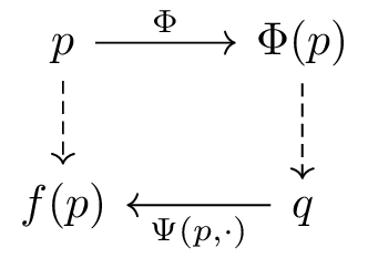
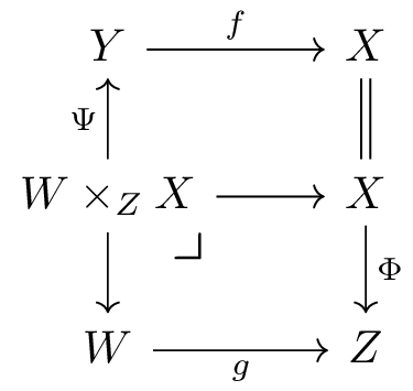
The upshot of the definition of Weihrauch reducible is that you have a “forward map” $\mathrm{\Phi }$ that converts inputs for $f$ to inputs for $g$, you solve your problem $g$, then convert your output of $g$ to an output of $f$ using a “backward map” $\mathrm{\Psi }$. When using the backward map, you also get to use the original input. This is summarised in the diagram below.

If you’ve seen lenses or other bidirectional mathematical structures, you get excited when you see things like this. However, as usual with computer science, there is a bunch of plumbing required to make everything fit, starting with a trip into realisability.

What is a PCA?

I will not be giving an in-depth treatment of Categorical Realisability, but for an introduction to the topic, you can read Tom de Jong's notes from a course that I had the pleasure of attending at MGS this year.

A PCA, or Partial Combinatory Algebra if you're not into the whole brevity thing, is a set $A$ of “combinators” and a partial operator called “application”, $\cdot :\subseteq A\times A\to A$, plus two special combinators called $S$ and $K$ satisfying a few axioms. We will not dwell on this, because we have a lot to get through, but these $S$ and $K$ are the combinators you would get from a process called bracket abstraction in the untyped lambda calculus. They are “combinatorially complete” which means any term built out of application, variables, and elements of $A$ can be expressed solely through application and $K$ and $S$.

There are lots of examples of PCAs, from the trivial $\{\star \}$ to the not-so-trivial untyped lambda calculus. We will skip Kleene's first model to his second model ${\mathcal{K}}_2$.

What is Kleene's Second Model?

Kleene's Second model is the PCA that corresponds to Type 2 Computability, which is the setting for much of Computable Analysis in general and Weihrauch Reducibility in particular. So, what is type 2 computability?

There are a few things to notice. First, we will usually view these functions $\alpha \in {\mathbb{N}}^{\mathbb{N}}$ as sequences of natural numbers. Second, we are taking the whole space of functions ${\mathbb{N}}^{\mathbb{N}}$ as our input, which means that some of our inputs are not computable; this is intentional. Finally, a consequence of this definition is that our function is continuous, in that $f(n)$ will be written to the output tape after finite time after inspecting only a finite prefix of the input.

To form a PCA, we want to take ${\mathbb{N}}^{\mathbb{N}}$ as our set of objects and define a multiplication map. It's a little fiddly, e.g., see section 1.4.3 of van Oosten's book, but I will provide a short explanation based on a nice answer on mathoverflow.

Fix a function $\alpha :{\mathbb{N}}^{\mathbb{N}}\to {\mathbb{N}}^{\mathbb{N}}$. We will instead view this as a function $\alpha :{\mathbb{N}}^{\mathbb{N}}\times \mathbb{N}\to \mathrm{Maybe}\mathbb{N}$, by uncurrying and fixing an isomorphism $N\cong N+\mathrm{\perp }$.

The first step is to define a partial map $F_{\alpha }:\subseteq {\mathbb{N}}^{\mathbb{N}}\to \mathrm{Maybe}\mathbb{N}$ by repeatedly running $\alpha ({\beta }_0,\dots ,{\beta }_n)$ on an input sequence $\beta \in {\mathbb{N}}^{\mathbb{N}}$, increasing $n$ each time, until we get a non-$\mathrm{None}$ answer $\mathrm{Just}k$. If this happens, return it; if the loop never terminates or $\alpha$ diverges on some input, return $\mathrm{None}$. That is, we keep asking for more of $\beta$ until we have enough for $\alpha$ to compute the answer. It turns out that every continuous partial function ${\mathbb{N}}^{\mathbb{N}}\to \mathbb{N}$ is equal to such an $F_{\alpha }$ for some $\alpha$.

Now we can define multiplication by $(\alpha \cdot \beta )(n)=F_{\alpha }(n,\beta )$, provided the right side is defined for all $n$.

There is a (non-runnable) Haskell pseudo-implementation provided below for the people who prefer code to prose.

Finally, ${\mathcal{K}}_2^{\mathrm{rec}}$ is the sub-PCA of ${\mathcal{K}}_2$ where all elements $\alpha \in {\mathbb{N}}^{\mathbb{N}}$ are recursive

What is the Category $\mathsf{\text{Pasm}}({\mathcal{K}}_2^{\mathrm{rec}},{\mathcal{K}}_2)$?

Assemblies

Now that we understand PCAs, we can define the notions of assembly and tracking, then form a category from assembly maps. The following definitions come straight from Tom's notes.

The standard analogy is to think of $a⊩x$ as telling us that $a$ is an implementation of $x$ in the PCA and that trackers implement their respective functions in the PCA.

Assembly maps form a category $\mathsf{\text{Asm}}(\mathcal{A})$, since the identity function can be tracked by the element $(S\cdot K)\cdot K$, and composition of functions is tracked by composition of trackers in a suitable sense. Again, I defer to Tom's notes in the desire to save space and time.

Specialising these notions to ${\mathcal{K}}_2$, we get that represented spaces are the same thing as assemblies and an element $\alpha \in {\mathbb{N}}^{\mathbb{N}}$ that tracks a function $f$ is a realiser for it.

However, the category just described would not be fully faithful to the notion of Type 2 Computability if you just instantiated it on either ${\mathcal{K}}_2$ or ${\mathcal{K}}_2^{\mathrm{rec}}$. This is because, as mentioned earlier, in Type 2 we want our computation to be performed by Turing machines, but to allow the sequences on our input tapes to be arbitrary, and hence possibly uncomputable. This suggests that the objects of our category should be assemblies on ${\mathcal{K}}_2$, but that our trackers should be required to come from the sub-assembly ${\mathcal{K}}_2^{\mathrm{rec}}$. This would give us a category $\mathsf{\text{Asm}}({\mathcal{K}}_2^{\mathrm{rec}},{\mathcal{K}}_2)$.

Partitioned Assemblies

The next important definition is that of a partitioned assembly. This is simply an assembly where each element of the set is realised by a unique element of the PCA.

In Computable Analysis, it is common to work with ${\mathbb{N}}^{\mathbb{N}}$ directly rather than with represented sets. In this setting, you can think of elements of ${\mathbb{N}}^{\mathbb{N}}$ as coding themselves one-to-one. I'm sure it's clear how to do it, but I will do it for completeness. Given a problem $f:\subseteq X\rightrightarrows Y$, we set $X^{\prime }=\mathrm{dom}({\delta }_X)$, $Y^{\prime }=\mathrm{dom}({\delta }_X)$ and define a new problem $f^{\prime }:\subseteq X^{\prime }\rightrightarrows Y^{\prime }$ by $(x,y)\in f^{\prime }⟺({\delta }_X(x),{\delta }_Y(y))\in f$.

Further, these problems are equivalent (Weihrauch reducible to one another) by taking the identity function as the forward map and the second projection as the backward map.

Finally, we can say that $\mathsf{\text{Pasm}}({\mathcal{K}}_2^{\mathrm{rec}},{\mathcal{K}}_2)$ is the category of partitioned assemblies over ${\mathcal{K}}_2$, where each map is tracked by an element of ${\mathcal{K}}_2^{\mathrm{rec}}$. Hopefully you agree by now that this is an appropriate category for handling Weihrauch reducibility, but there is one last snag to deal with.

Weihrauch Problems are Bundles

The definition of reducibility above relates partial multi-valued functions (a.k.a. problems) to each other. However, the maps in our category are tracked functions, so they are not a good fit. What gives?

Another way of viewing a problem $f:\subseteq X\rightrightarrows Y$ is as a family of sets ${\left(Y_x\right)}_{x\in X}$ where $Y_x=\{y\in Y:(x,y)\in f\}$. In the language of dependent types, we might say there is a type family $Y(x)$ indexed by $X$ and form a dependent sum $\sum _{x:X}Y(x)$. This type has a projection function, ${\pi }_X:\sum _{x:X}Y(x)\to X$ which maps “answers” to the “instance” of the problem they solve. Since we have defined it using dependent types, the projection map is total and tracked, which means ${\pi }_X$ is an arrow in $\mathsf{\text{Pasm}}({\mathcal{K}}_2^{\mathrm{rec}},{\mathcal{K}}_2)$. Such maps are known as bundles.

One final thing to note about ${\pi }_X$ is that it is not necessarily surjective; specifically, its image is $\mathrm{dom}(f)$. It is typical in computable analysis to assume that all problem instances have solutions, but everything I will say below also works in the non-total case.

That's all very well and good but what about Lenses?

When I think of lenses, I normally think of the $\mathsf{\text{Poly}}$, the category of polynomial functors, where (dependent) lens is just another name for a natural transformation. However, this category is defined in terms of $\mathsf{\text{Set}}$ rather than $\mathsf{\text{Pasm}}({\mathcal{K}}_2^{\mathrm{rec}},{\mathcal{K}}_2)$. The good news is that Gambino & Kock worked out the theory of polynomial functors back in 2010 for arbitrary locally cartesian closed categories; the bad news is that $\mathsf{\text{Pasm}}({\mathcal{K}}_2^{\mathrm{rec}},{\mathcal{K}}_2)$ is not locally cartesian closed (only weakly so).

In the rest of this section, we will borrow enough of Gambino & Kock to try and justify the “is a lens” claim.

Polynomials

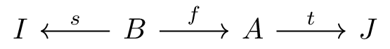
A polynomial over a locally cartesian closed category $\mathcal{E}$ with a terminal object is a diagram $F$ in $\mathcal{E}$ of shape:

The intent of this definition is to capture the concept of a $J$-indexed family of polynomials in $I$-many variables. In the case of a single polynomial in one variable, we can specialise this by taking $I=J=1$, where $1$ is the terminal object. Thus, a polynomial is “just” an arrow $f:B\to A$. More specifically, taking the dependently typed view from earlier, a problem / polynomial $f$ given by a type $\sum _{a:A}B(a)$ and its projection function ${\pi }_A$.

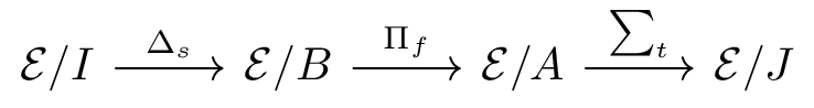
Polynomial Functors

In a locally cartesian closed category, we would then go on to define a polynomial functor $P_F:\mathcal{E}/I\to \mathcal{E}/J$ as the composite

where ${\mathrm{\Delta }}_s$ is pullback along $s$, $\sum _t⊣{\mathrm{\Delta }}_t$ is the “Dependent Sum” functor and ${\mathrm{\Delta }}_f⊣{\mathrm{\Pi }}_f$ is the “Dependent Product” functor. The first adjunction is well-defined in any category with pullbacks. The second adjunction, on the other hand, is only defined in a locally cartesian-closed category. Since Pasm isn't an LCCC, we will skip on and not worry about what all this means. Maybe another day…

Lenses

So we don't have an LCCC, but we do have pullbacks in $\mathsf{\text{Pasm}}({\mathcal{K}}_2^{\mathrm{rec}},{\mathcal{K}}_2)$ and this will turn out to be enough to define lenses. First, we will blithely skip about ten pages further along in G&K's paper to this lovely theorem.

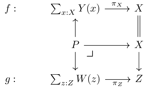
Every strong natural transformation $P_F\Rightarrow P_G$ between polynomial functors is represented in an essentially unique way by a diagram like:

Now, this is something we can work with. This diagram expresses that morphisms between polynomial functors have a vertical-cartesian factorisation system. Again, we don't need to worry too much about what that means here except to note that a cartesian natural transformation is one whose naturality squares are all pullbacks.

Now, let's simplify the diagram using $I=J=1$ and viewing problems $f:\subseteq X\rightrightarrows Y$, $g:\subseteq Z\rightrightarrows W$ as bundles.

If we wanted to fill in this diagram in $\mathsf{\text{Pasm}}({\mathcal{K}}_2^{\mathrm{rec}},{\mathcal{K}}_2)$ such that both squares commute, what work would we need to do? $\mathsf{\text{Pasm}}({\mathcal{K}}_2^{\mathrm{rec}},{\mathcal{K}}_2)$ has pullbacks, so once we have an arrow $\mathrm{\Phi }:X\to Z$ we'd have the bottom square. What would such a pullback look like? The construction of pullbacks in $\mathsf{\text{Pasm}}({\mathcal{K}}_2^{\mathrm{rec}},{\mathcal{K}}_2)$ is exactly like that in $\mathsf{\text{Set}}$ (except for some additional information about realisers and arrows being tracked), so we can take $P=\sum _{x:X}W(\mathrm{\Phi }(x))$ with the obvious morphisms ${\pi }_X:P\to X$ and $(x,w)\mapsto (\mathrm{\Phi }(x),w):P\to \sum _{z:Z}W(z)$.

Now that we know $P$, we can determine what needs to be true of the remaining arrow $\mathrm{\Psi }:P\to \sum _{x:X}Y(x)$ for the top square to commute. Let $x\in X$, $w\in W(\mathrm{\Phi }(x))$, then ${\pi }_X(\mathrm{\Psi }(x,w))={\pi }_X(x,w)=x$, so $\mathrm{\Psi }(x,w)=(x,y)$ for some $y\in Y(x)$. In other words, $\mathrm{\Psi }(x,\cdot )$, is a map $W(\mathrm{\Phi }(x))\to Y(x)$.

I claim that these $\mathrm{\Phi }$ and $\mathrm{\Psi }$ are the same as those from earlier but recast in the new language. First, since we are working with partitioned assemblies, we take all the coding maps $\delta$ to be the identity. Next, we view a problem $f:\subseteq X\rightrightarrows Y$ as a bundle ${\pi }_X:\sum _{x:X}Y(x)\to Y$ and recall that the image of ${\pi }_X$ is $\mathrm{dom}(f)$. Then saying that a computable function $\mathrm{\Phi }:X\to Y$ takes $x\in \mathrm{dom}(f)$ to $\mathrm{\Phi }(x)\in \mathrm{dom}(g)$ is the same as saying that the lower half of the diagram is a pullback square. Finally, the requirement that $y\in g(\mathrm{\Phi }(x))$ implies that $\mathrm{\Psi }(x,y)\in f(x)$ is the same as saying that $(\mathrm{\Phi }(x),y):\sum _{z:Z}W(z)$ implies $(x,\mathrm{\Psi }(x,y)):\sum _{x:X}Y(x)$. Looking only at the second arguments, we see that this means we require a function $\mathrm{\Psi }(x,\cdot ):W(\mathrm{\Phi }(x))\to Y(x)$.

Finally, we can make the following definitions.

Given (extended) problems $f:Y\to X$, $g:W\to Z$ in $\mathsf{\text{Pasm}}({\mathcal{K}}_2^{\mathrm{rec}},{\mathcal{K}}_2)$. Then f is Weihrauch Reducible to $g$, $f{\le }_{W}g$, if there exists arrows $\mathrm{\Phi }:X\to Z$, $\mathrm{\Psi }:W{\times }_{Z}X\to Y$ such that the following diagram commutes:

Wrapping up

So, we've managed to give another definition of Weihrauch Reducibility, but this note is already too long, so I'll have to leave a few things on the table. First, I haven't argued that these form a category of problems, of which the poset of Weihrauch degrees should be the skeleton. Second, I never showed that various operators on degrees correspond to familiar operators on polynomials. Lastly, I should mention my supervisors's most recent preprint, where she discusses the notion of extended Weihrauch reducibility.

Thanks must go, firstly, to my supervisor, Cécilia Pradic, for putting up with all the questions necessary for me to understand this topic. I should also thank the members of the Computable Analysis group at Swansea (Arno Pauly, Manlio Valenti, Eike Neumann), for what little I know about Weihrauch reducibility. I would have been in a bad place to even start this writeup if I hadn't attended Tom de Jong's Categorical Realisability course at MGS. Finally, thanks to the people I talked to at SPLV that were interested, since otherwise I might never have bothered to write it up.